On the Range of City Sizes

In the last post on carbon pricing, I mentioned that I had been planning on a post on Zipf’s law, which is a description of the distribution of city sizes with a country. And so here we go. This post is part of my Scaling in Human Societies project, supported by the Living Literature Review grant from OpenPhilanthropy, though this work represents my own views and not those of OpenPhil. This material can be found at the Scaling site, with some content that is not in the blog post.
I will confess that this post is not the easiest to write. While an interesting mathematical curiosity, the significance of Zipf’s law is far from clear, and this may be one of those observations for which there is less than meets the eye. I also cannot avoid that there are more mathematics than usual here, though I will try my best to keep it painless. Nevertheless, Zipf’s law does offer some valuable insight into the nature of urban growth.
Zipf’s Law
Zipf’s law, named for the linguist George Kingsley Zipf, is a general observation about the sorted values of quantities in a list. Zipf introduced the principle for linguistics in Zipf (1932) and expanded upon it in his book Zipf (1949).
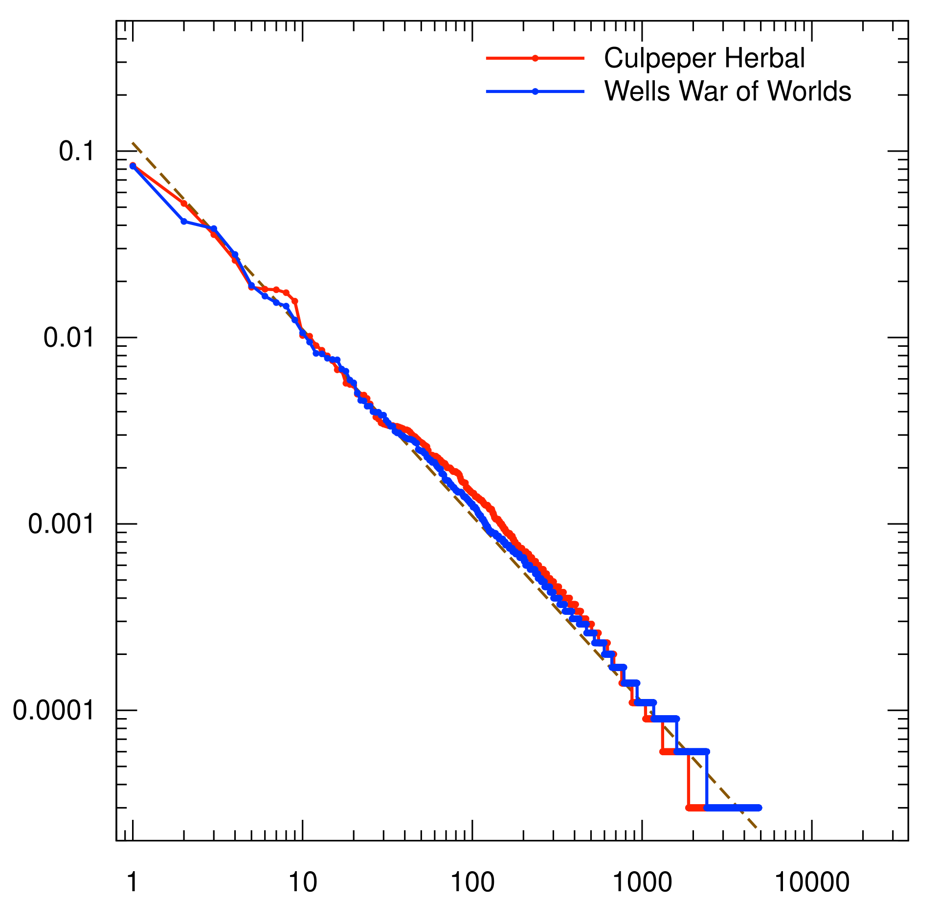
In linguistics, Zipf’s law concerns the distribution of words in a corpus. Order the words by frequency, so that the most common word comes first, followed by the second most common word, the third most common word, and so forth. Zipf’s law states that the frequency of a word should be inversely proportional to its rank order. In other words, the most common word appears twice as often as the second most common word, three times as often as the third most common word, and so forth.
Forms of Zipf’s law arise in many contexts. One of them, the distribution of city sizes within a country, is our main item of interest and will be addressed later. Another is in music, where Manaris et al. (2005) show how 40 parameters in compositions such as “pitch, duration, melodic intervals, and harmonic consonance” satisfy a Zipfian distribution. Louridas, Spinellis, and Vlachos (2008) show that Zipf-like power law distributions are pervasive in software engineering. Bender and Gill (1986) find that Zipf’s law holds in the DNA sequence of the bacterial virus ΦX174.
A power law is a more general distribution, given by P(S > x) = k/x^ξ. Here, S is our random variable, x is some threshold value, k is a constant, and ξ is the exponent associated with the distribution. The higher the value of ξ is, the more rare high outliers are. Zipf’s law is the particular case that ξ=1. Power law distributions themselves are common, such as in modeling the severity of epidemics, earthquakes, and wars, but this would be too much of a digression. Gabaix (2009) shows that power law distributions are pervasive in economics and finances.
Actually, the reader may notice a slight sleight of hand above. The rank/frequency property and the power law where ξ=1 are in fact the same distributions in an idealized sense, but the rank/frequency property is often expressed with reference to the largest frequency in the set, unlike the power law where ξ=1. This makes the power law formulation more robust to situations where the largest frequency(ies) are outliers, and thus, while a less intuitively clear expression, it is better to use for statistical analysis.
Zipf’s law is an example of Stigler’s Law of Eponymy (Stigler (1980)), which Stephen Stigler attributes to Robert Merton, that eponymous laws and principles are typically named after people who had, at most, a minor role in their development. The earliest variant of the rule that I have been able to find goes back to Pareto (1896) himself, where he finds that the distribution of wealth in a society follows a power law, though not necessarily with ξ=1.
There are far too many examples of Zipf’s law in physical systems to attempt to review, but now, let us turn to how this applies specifically to cities.
Zipf’s Law in City Sizes
For city sizes within a country (or any urban system where people can move about freely), Zipf’s law is a rank/size distribution. If the largest city in the system has a population of N, then the second largest city will have a population of N/2, the third largest city will have a population of N/3, and so on. As before, one can also formulate this in terms of a power law distribution.As another illustration of Stigler’s law of Eponymy, most papers attribute the earliest expression of Zipf’s law for cities to Auerbach (1913) (English translation), which finds that a Zipfian distribution holds in German cities in 1910.
Since then, many researchers have investigated the validity of Zipf’s law for cities, finding varying degrees to which the law fits the data. We’ll get to a bit of that, but first, let us understand how the law might arise.
The Origins of Zipf’s Law
When there is a statistical property that arises with such regularity, one seeks a general explanation for it. There are many candidates for that generation explanation. The one I will offer, following Gabaix (1999), is based on Gibrat’s law.
Posited in Gibrat (1931), Gibrat’s law models a scenario of many cities (firms in the original paper, but I’ll stick with cities) in a system whereby the distribution of proportional growth or decline rates of the cities is fixed. A simplified example given in Gabaix (1999) is that, for every time period, each city has a 1/3 chance of doubling in size and a 2/3 chance of halving in size. The proportional growth/decline rate does not depend on city size.
Gabaix (1999) shows that, under Gibrat’s law, the distribution of city sizes should converge to a Zipfian distribution, regardless of how it starts. To insure this, the additional assumption of a lower bound on city size is needed. This is sensible; a city obviously cannot have a population less than 1, assuming it exists at all.
A good analogue, and one that will be a bit more familiar, is the central limit theorem. The CLT holds that, given n identical and independent random variables with mean μ and finite standard deviation σ², the sample mean converges to a normal (i.e. Bell curve) distribution as n→∞, regardless of what the original distributions look like. There are any number of precise expositions and proofs of the CLT, such as Kwak and Kim (2017), but I want to avoid any more mathematical detail than necessary.
The “identical” assumption above can be relaxed quite a bit, though not arbitrarily. And yet, as Lyon (2014) discusses, normal distributions arise in many, many places in nature where the central limit theory clearly would not apply, such as in the distribution of heights or the sizes of snowflakes. Lyon gives an explanation in terms of maximizing entropy instead; read the paper if you really want the details. The relevance for Zipf’s law is that, while Gibrat’s law may be an intuitive explanation for how Zipf’s law arises, we may still expect to see the Zipfian pattern even when there is no obvious proportional growth mechanism.
Gabaix (1999) goes on to show that the growth rate of cities can vary—for instance, some cities might have higher growth because of geographic or cultural advantages—so long as the proportional growth rate does not depend on the current size. He also allows for new cities to appear, so long as the rate of new city formation is less than the growth rate of the whole society. These assumptions allow Zipf’s law to arise in situations that are a bit more realistic. Still, Gabaix does not break away from the proportional growth model.
Empirical Results
OK, thank you for bearing with a load of theory. Now let us see how well Zipf’s law actually performs. There are very many studies on this topic, and so we are only going to consider a few of them.
Starting with Gabaix (1999) again, he considers 135 metropolitan regions in the United States, based on 1991 data, and applies a regression to the natural log of rank in terms of the natural log of size. The slope of the line is -1.005 and the R² value is 0.986. Recall that an idealized Zipfian distribution has a slope of -1, and so this is a remarkably good fit.
I argued last year that metropolitan regions are more relevant than cities as defined by administrative boundaries. A metropolitan region, defined roughly as unified labor market that corresponds to an average ~30 minute commutershed, corresponds to a city in the sense that most people experience it, whereas people generally experience administrative cities as arbitrary delineations. I currently live in the city of Beaverton, Oregon, in the Portland metro area. I don’t even know where the borders are with Portland, Aloha, Hillsboro, Tigard, and unincorporated Washington County, nor are they relevant to me for any purpose other than voting and taxes. Unfortunately, since data tends to be more available for administrative cities rather than urban agglomerations (an international term for what we Americans call metropolitan regions), that’s what we often have.
Soo (2005) takes an international view of Zipf’s law and finds a less convincing picture than Gabaix (1999). He considers both administrative cities and urban agglomerations, and while there is more focus in the paper on the former, I want to focus on the latter for reasons outlined above.
Soo (2005) considers 29 countries for which data on urban agglomerations are available. He then estimates the exponent of the fit pareto distribution. Considering two estimates—ordinary least squares and the Hill estimator (the distinction between the two is explained in the paper and not something we need to discuss here)—he estimates the exponent at 0.870 and 0.8782 respectively. The exponent would be 1.0 in an ideal Zipf distribution. The fact that it is found to be well less than 1 indicates that the distribution is flatter than an ideal Zipf distribution, or in other words, there are more large metros than one would expect from a pure Gibrat growth process.
Looking at individual countries, Soo (2005) finds that in 16 of 29 countries with data, the exponent is significantly less than one. In only two countries, the exponent is significantly greater than 1. In the rest, the exponent is statistically indistinguishable from 1. Soo finds roughly the opposite of all this when considering administrative cities, but as I argued above, urban agglomerations are a more useful basis of comparison.
The following is not Soo's (2005) interpretation, but rather my own. If we were to model a growth process analogous to Gibrat’s law, then it must be that growth is biased so that larger agglomerations generally see higher proportional growth rates than smaller metros, and thus over time, population becomes more concentrated in larger metros. This is what one would expect from agglomeration economies: larger metros provide better job opportunities than smaller metros, and so they are more favored to grow than smaller metros.
We could better evaluate this hypothesis if we had an analysis of population data for urban agglomerations across countries and over time, so that we could see the growth rates more directly. Perhaps such an analysis exists, but I am not aware of it.
Dittmar (2011) offers a contrasting result. He considers historical population sizes in cities in Western Europe from 1300 to 1800. Considering all cities that ever had a population of at least 5000 people over this time, Dittmar finds that a Zipf distribution fits poorly before 1500, and after 1500, the fit is generally good. Prior to 1500, there are too few large cities relative to what would be expected from an ideal Zipf distribution. This is the opposite situation to what is described in Soo (2005), who finds more large urban agglomerations than would be expected from a Zipf distribution.
Dittmar's (2011) interpretation is that in the Middle Ages, city growth was constrained by land and transportation logistics—a city cannot be larger than the ability of the transportation system to provide food—and so growth of the larger cities was constrained relative to what would be expected from Gibrat’s law. These constraints were lifted by the early modern period, and so a Zipf distribution could take hold.
Conclusions
At the start, I said that there is less than meets the eye to Zipf’s law for city sizes. The main problem is that, despite decades of interest and an abundance of data, there is no consensus in the literature as to whether Zipf’s law really is the best model for city sizes, why this pattern arises, and even whether it arises for any reason other than statistical artifice.
Even if Zipf’s law is a good model, there is nothing normative about it. We cannot say from it how many big and small cities there “should” be, any more than we can conclude that the present distributions of height or IQ in the population is what they “should” be. I have discussed other city growth patterns before, such as Machetti’s constant and the standard urban model, and while these models have their own shortcomings, at least they have a basis in simple and rational economic processes. The same cannot be said for Zipf’s law.
However, it is undeniably true that there is no single ideal city size, and that a variety of city sizes is necessary for a society, even if that variety does not conform to a Zipfian distribution. Alain Bertaud’s Order Without Design (2018) makes this point well. Law firms specializing in international trade need a wide range of easy business connections and not a lot of space, and so you will find them in the largest cities. Farms need a lot of space and do not benefit much from agglomeration, and so you will find them in rural areas. Furniture factories occupy an intermediate position.
Diving into this subject has been an exercise in humility. Those of us who think a lot about cities are full of ideas about how they could be designed better. But there is much that we do not understand well.
Quick Hits
Marchetti’s constant is another example of Stigler’s Law of Eponymy. The earliest exposition I have found comes from Lewis Mumford’s 1934 Technics and Civilization, where he states that an increase in travel speed will manifest as increased travel distance rather than decreased travel time. Mumford, in turn, credits the observation to Bertrand Russell, though without referring to something written. This may be a concept whose origin is deep in the misty recesses of time. In the same discussion, Mumford asserts that improved communications technology—the telephone and typewriters in his day—manifests itself as an increased volume of communication rather than saved communication time, and furthermore, decreasing marginal value of the material being communicated effectively cancels the gains from technology. Both are rather cynical viewpoints, but contemporary office workers will likely suspect that there is some truth to them.
Those who are watching developments in autonomous weaponry should pay attention to the state of drone warfare in the Russia/Ukraine war. In June, the Institute for the Study of War analyzed the ways in which battlefield AI is still short of many commentators expect. This analysis was published a day after Operation Spiderweb, Ukraine’s spectacular attack of five Russian airbases, which is not mentioned.